Lesson 8:
Geographically Weighted Regression

Author

Affiliation

Dr. Kam Tin Seong
Assoc. Professor of Information Systems(Practice)

School of Computing and Information Systems,
Singapore Management University

Published

12 Mar 2023

Content

Introducing Regression Modelling
- Simple Linear Regression
- Multiple Linear Regression
What is Spatial Non-stationary
Introducing Geographically Weighted Regression
- Weighting functions (kernel)
- Weighting schemes
- Bandwidth
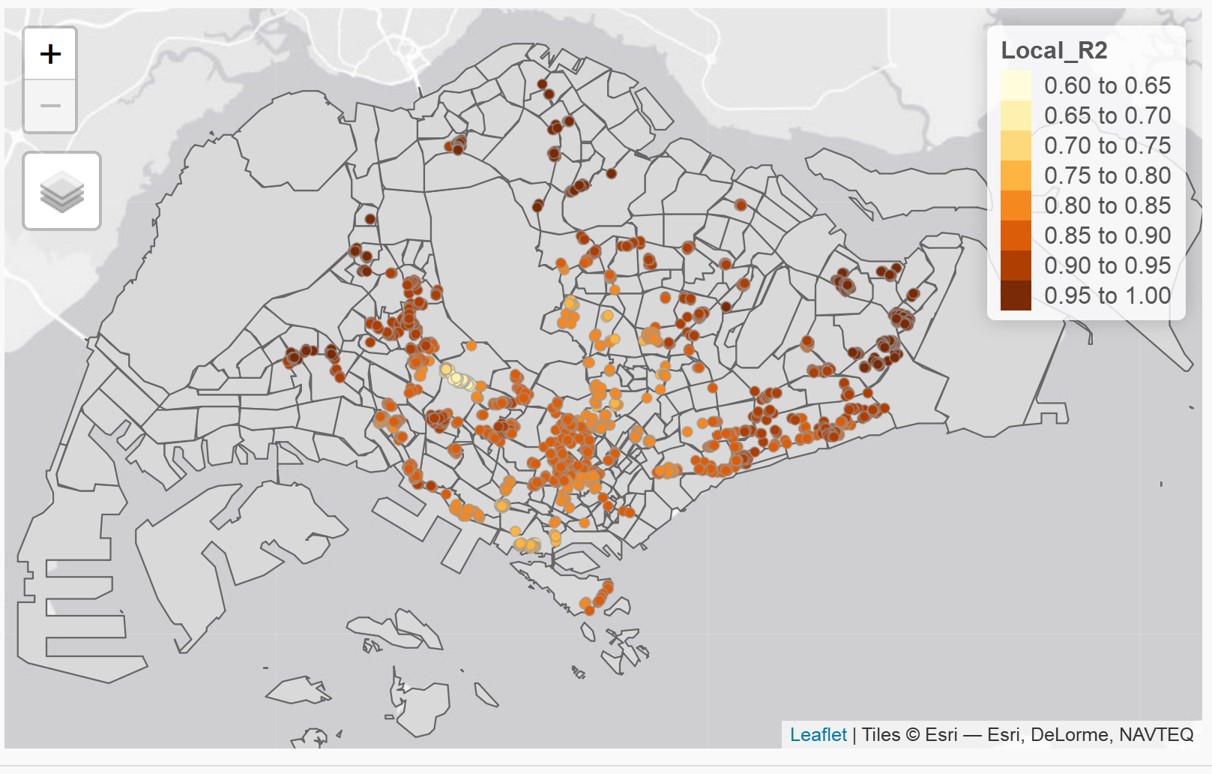
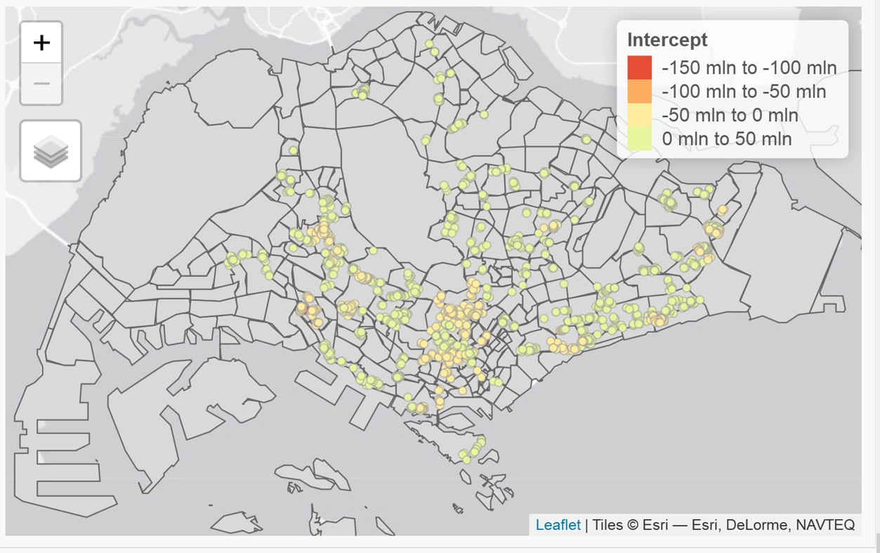
Interpreting and Visualising

The WHY Questions

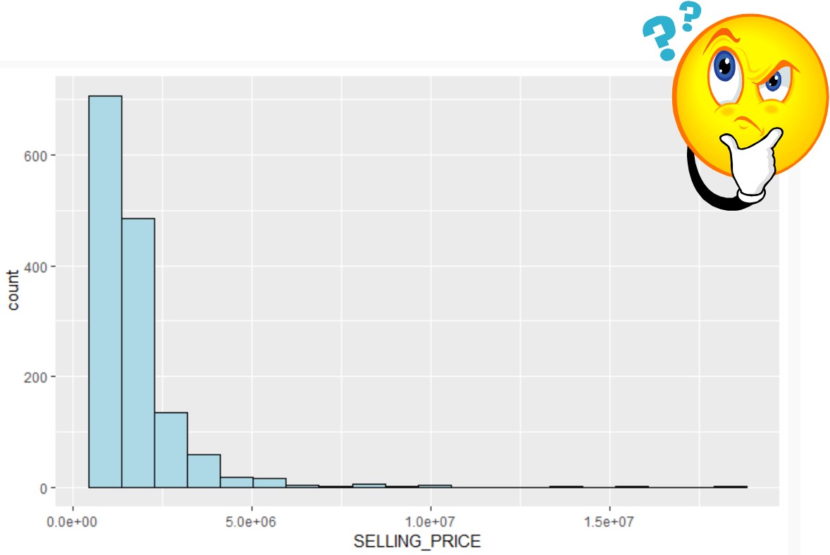
Why some condominium units were transacted at relatively higher prices than others?

The WHY Questions

Why condominium units located at the central part of Singapore were transacted at relatively higher prices than others?

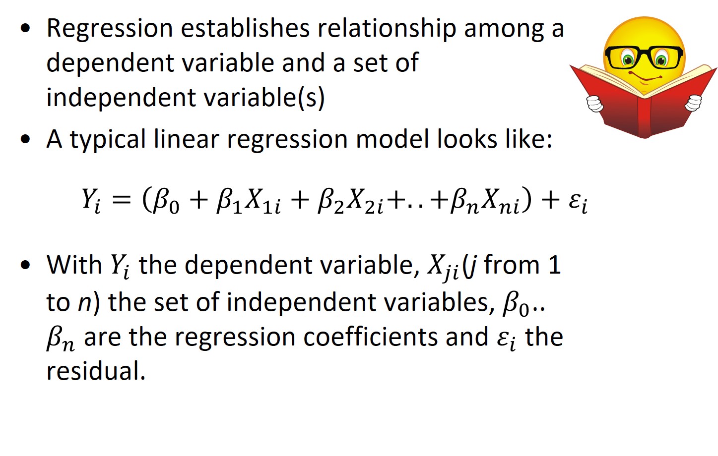
What is regression analysis?

A set of statistical processes for explaining the relationships among variables.
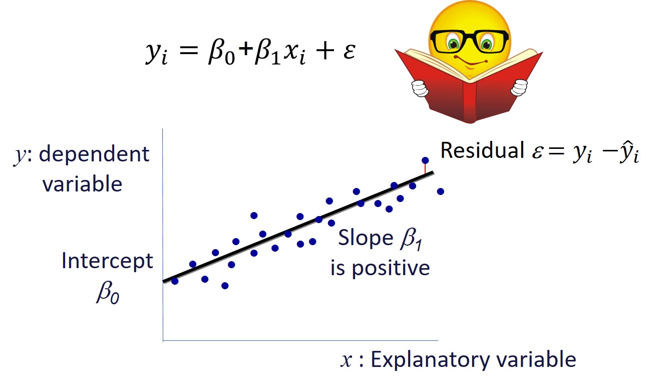
The focus is on the relationship between a dependent variable (y) and one or more independent variables (x)
- Does X affect Y? If so, how?
- What is the change in Y given a one unit change in X?
Estimate outcomes based on the relationships modelled.

A Simple Linear Regression Model

The formula:

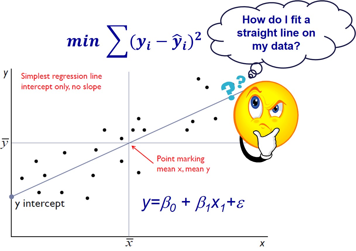
The Least Squares Method

The sum of the vertical deviations (y axis) of the points from the line is minimal.

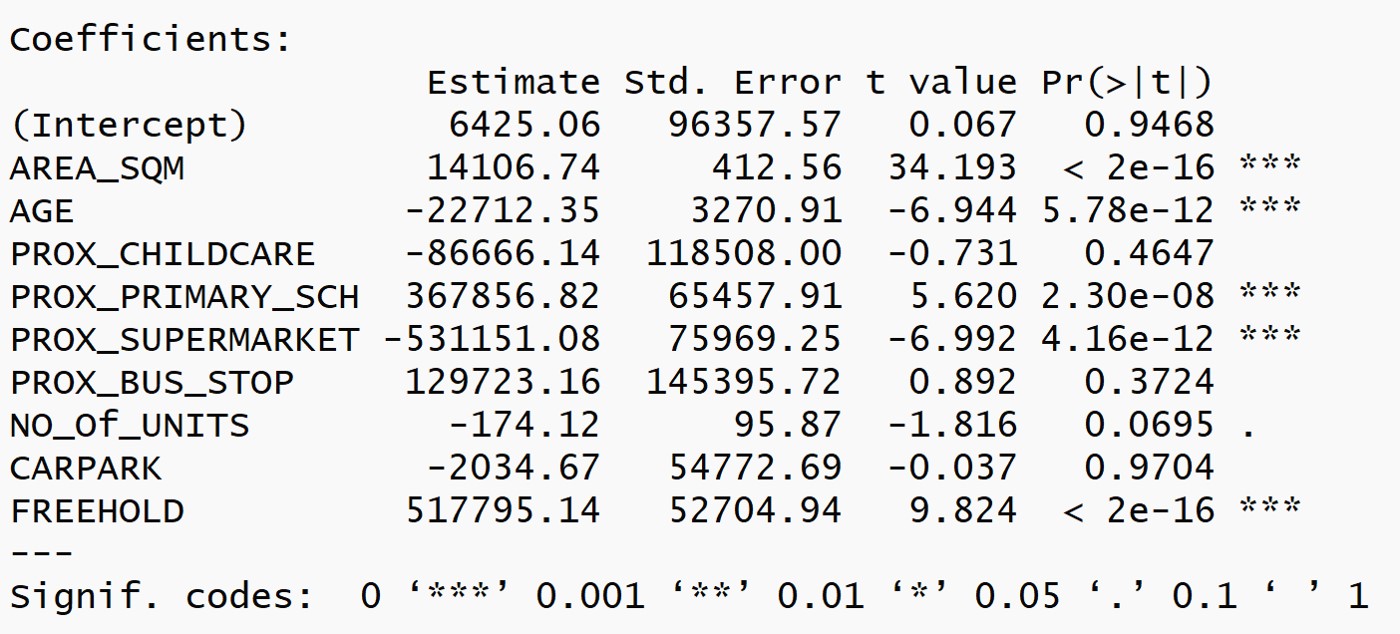
Multiple Linear Regression

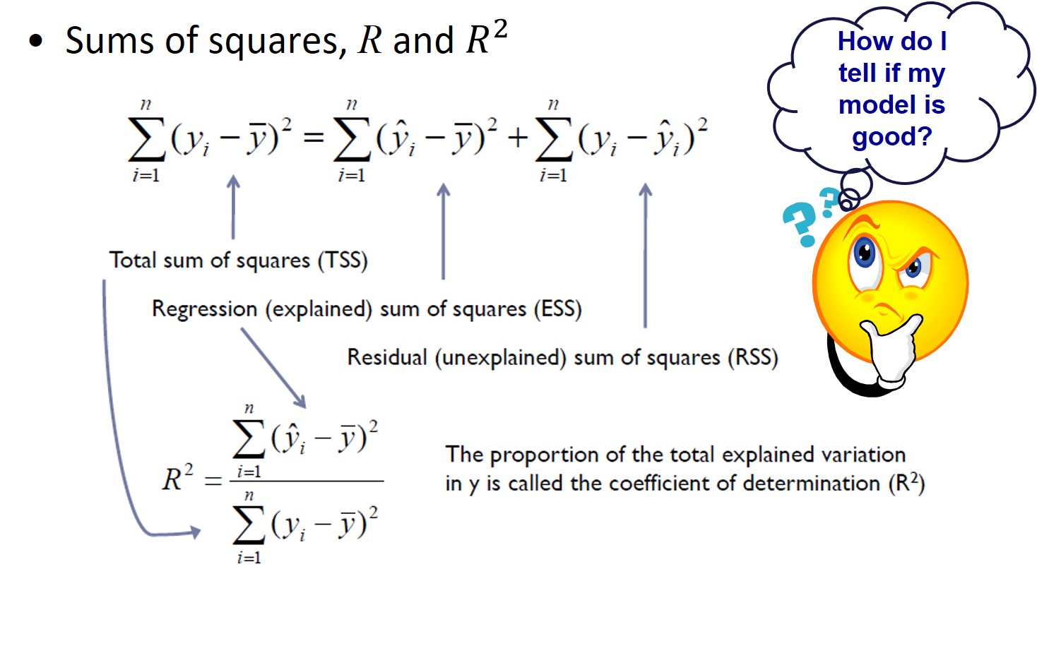
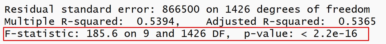
Assessing the goodness of fit

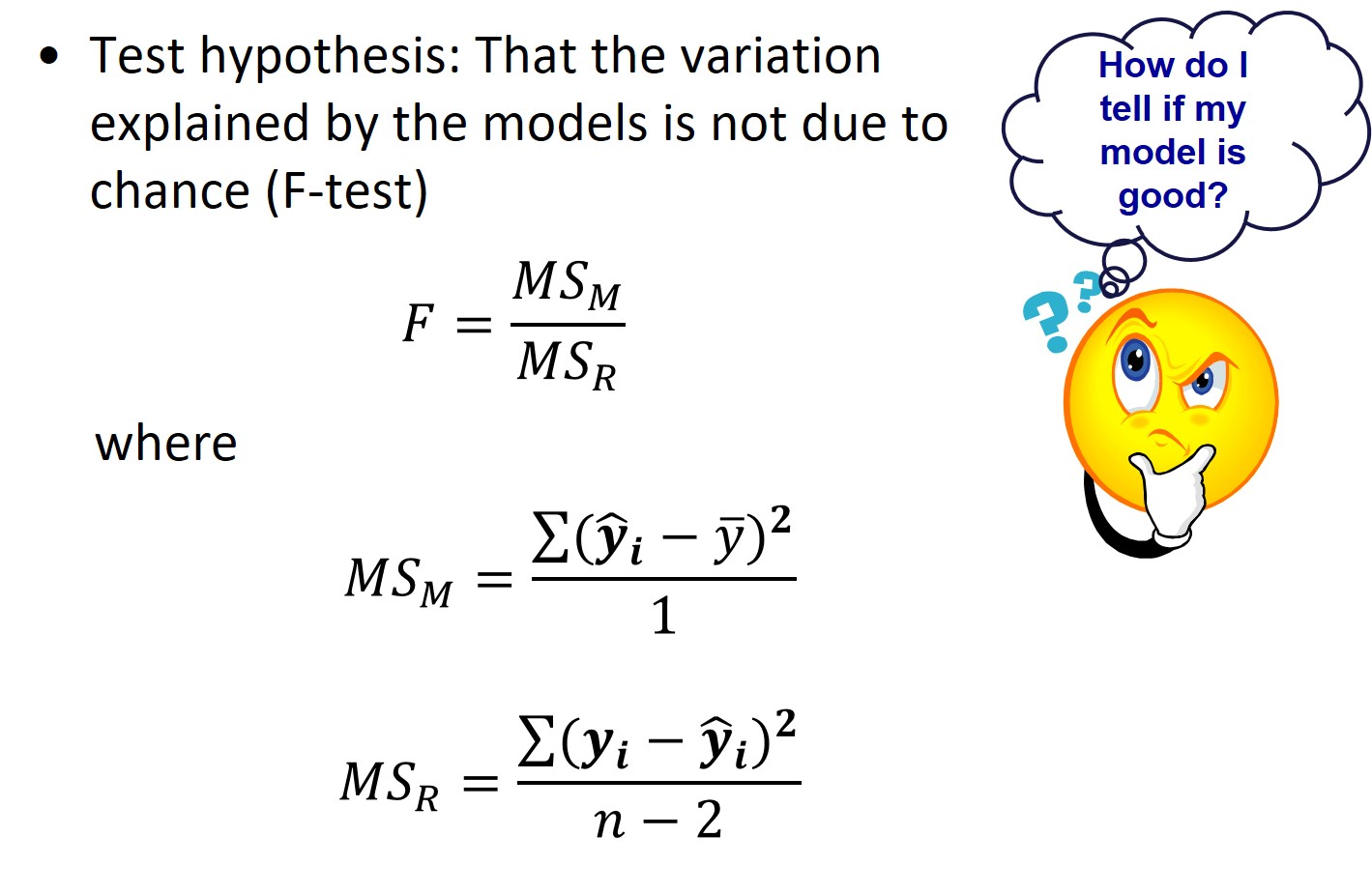
Significance testing in regression

Goodness of fit test

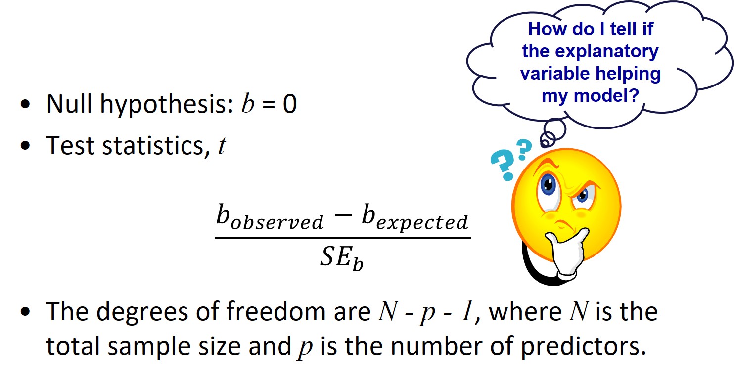
Individual parameter testing

Assessing individual parameters

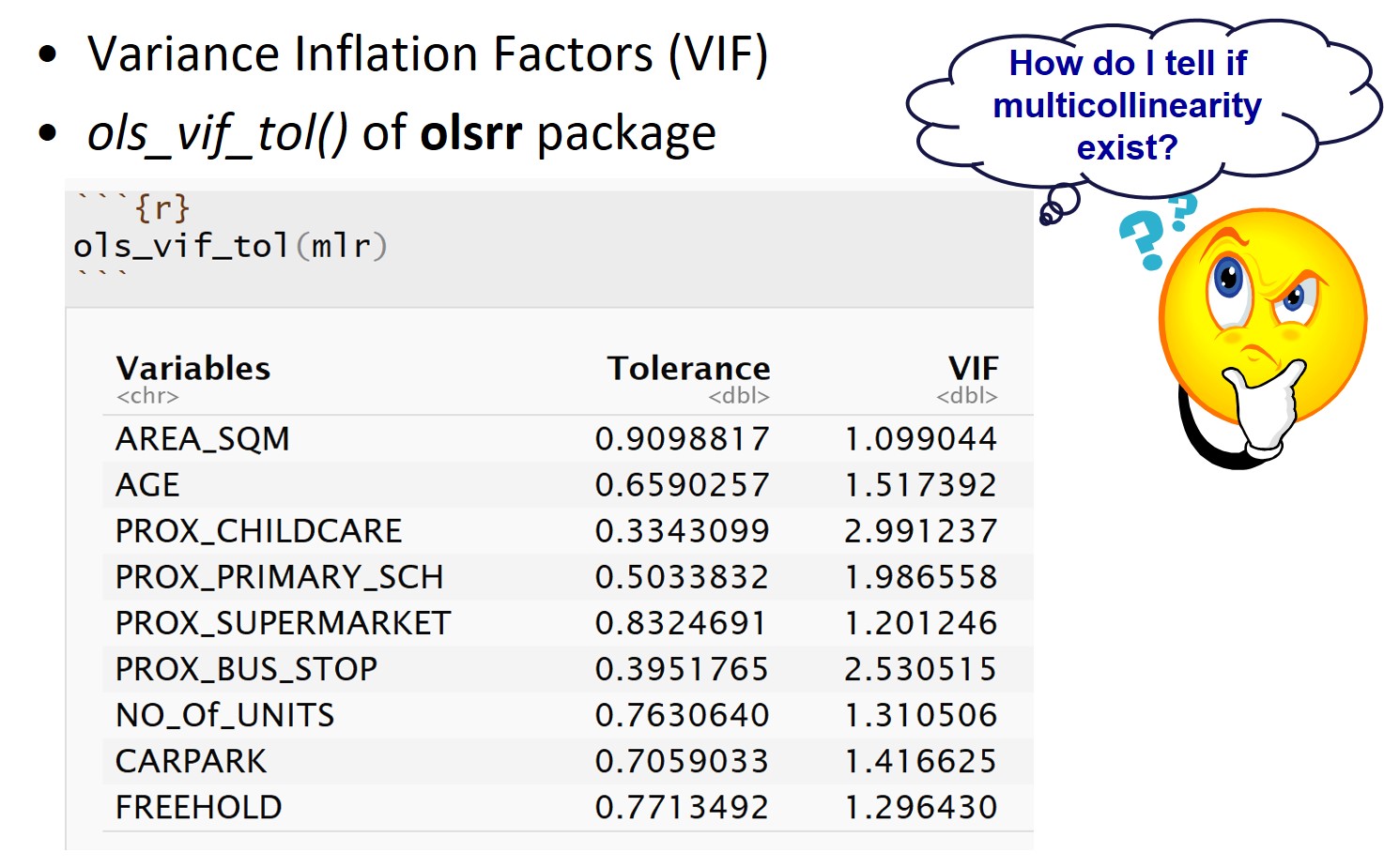
Are there redundant explanatory variables?

Assumptions of linear regression models

Linearity assumption. The relationship between the dependent variable and independent variables is (approximately) linear.
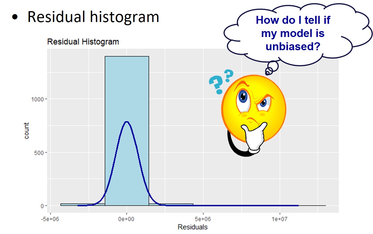
Normality assumption. The residual errors are assumed to be normally distributed.
Homogeneity of residuals variance. The residuals are assumed to have a constant variance (homoscedasticity).
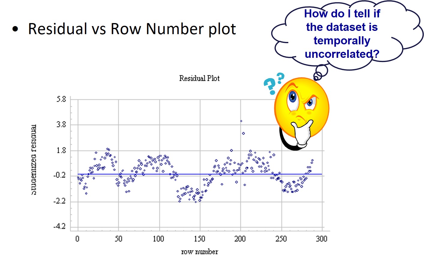
The residuals are uncorrelated with each other.
- serial correlation, as with time series
(Optional) The errors (residuals) are normally distributed and have a 0 population mean.]

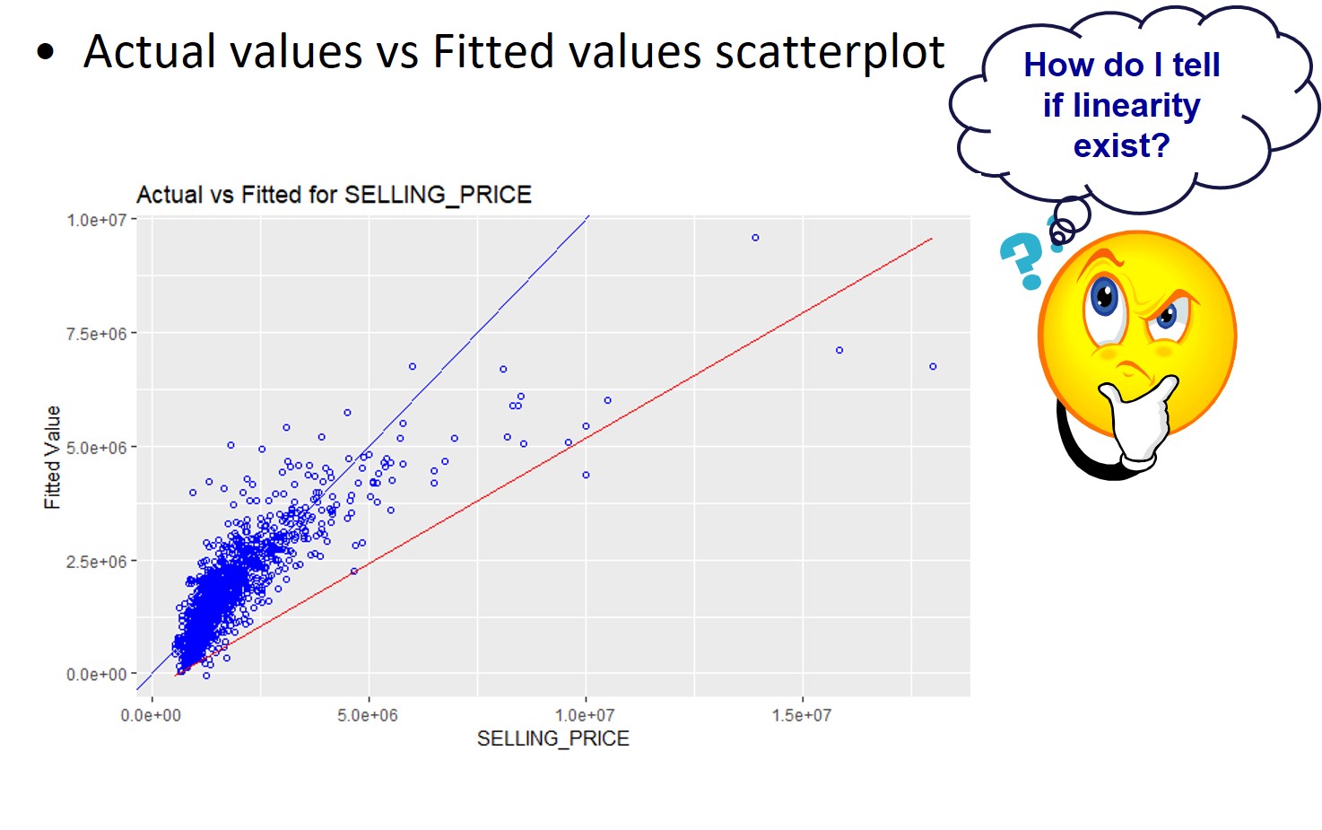
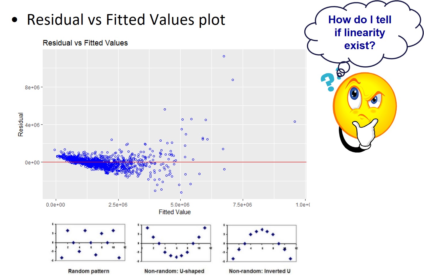
The linearity assumption

Residuals vs Fitted plot - Used to check the linear relationship assumptions. A horizontal line, without distinct patterns is an indication for a linear relationship, what is good.

Demystifying the linearity assumption myth

The myth: - We should transform the values of the y variable when they are large.

library(tidyverse)

── Attaching packages ─────────────────────────────────────── tidyverse 1.3.2 ──
✔ ggplot2 3.4.1     ✔ purrr   1.0.1
✔ tibble  3.1.8     ✔ dplyr   1.1.0
✔ tidyr   1.3.0     ✔ stringr 1.5.0
✔ readr   2.1.4     ✔ forcats 1.0.0
── Conflicts ────────────────────────────────────────── tidyverse_conflicts() ──
✖ dplyr::filter() masks stats::filter()
✖ dplyr::lag()    masks stats::lag()

library(sjPlot)
library(sjmisc)


Attaching package: 'sjmisc'

The following object is masked from 'package:purrr':

    is_empty

The following object is masked from 'package:tidyr':

    replace_na

The following object is masked from 'package:tibble':

    add_case

library(sjlabelled)


Attaching package: 'sjlabelled'

The following object is masked from 'package:forcats':

    as_factor

The following object is masked from 'package:dplyr':

    as_label

The following object is masked from 'package:ggplot2':

    as_label

library(olsrr)


Attaching package: 'olsrr'

The following object is masked from 'package:datasets':

    rivers

data1 <- read_delim("data/ex1_data.txt", delim=";")

Rows: 100 Columns: 3
── Column specification ────────────────────────────────────────────────────────
Delimiter: ";"
chr (1): group
dbl (2): x, y

ℹ Use `spec()` to retrieve the full column specification for this data.
ℹ Specify the column types or set `show_col_types = FALSE` to quiet this message.

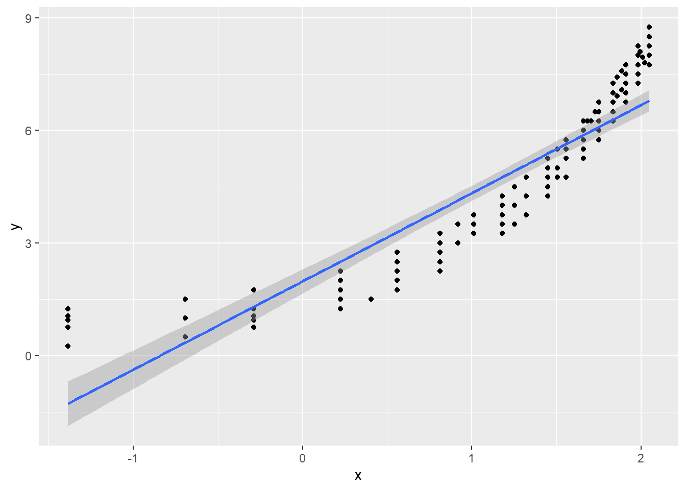
data1.lm <- lm(formula=y ~ x, data = data1)
tab_model(data1.lm)

	y
Predictors	Estimates	CI	p
(Intercept)	1.98	1.66 – 2.30	<0.001
x	2.35	2.13 – 2.57	<0.001
Observations	100
R² / R² adjusted	0.819 / 0.817

ggplot(data=data1,  
       aes(x=`x`, y=`y`)) +
  geom_point() +
  geom_smooth(method = lm)

`geom_smooth()` using formula = 'y ~ x'

The linearity assumption

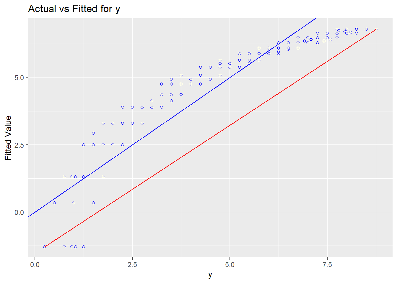
Despite the values of the dependent variable is rather similar to the values of the independent variable, the diagnostic plot shows that the linearity assumption has been violated.

ols_plot_obs_fit(data1.lm, print_plot = TRUE)

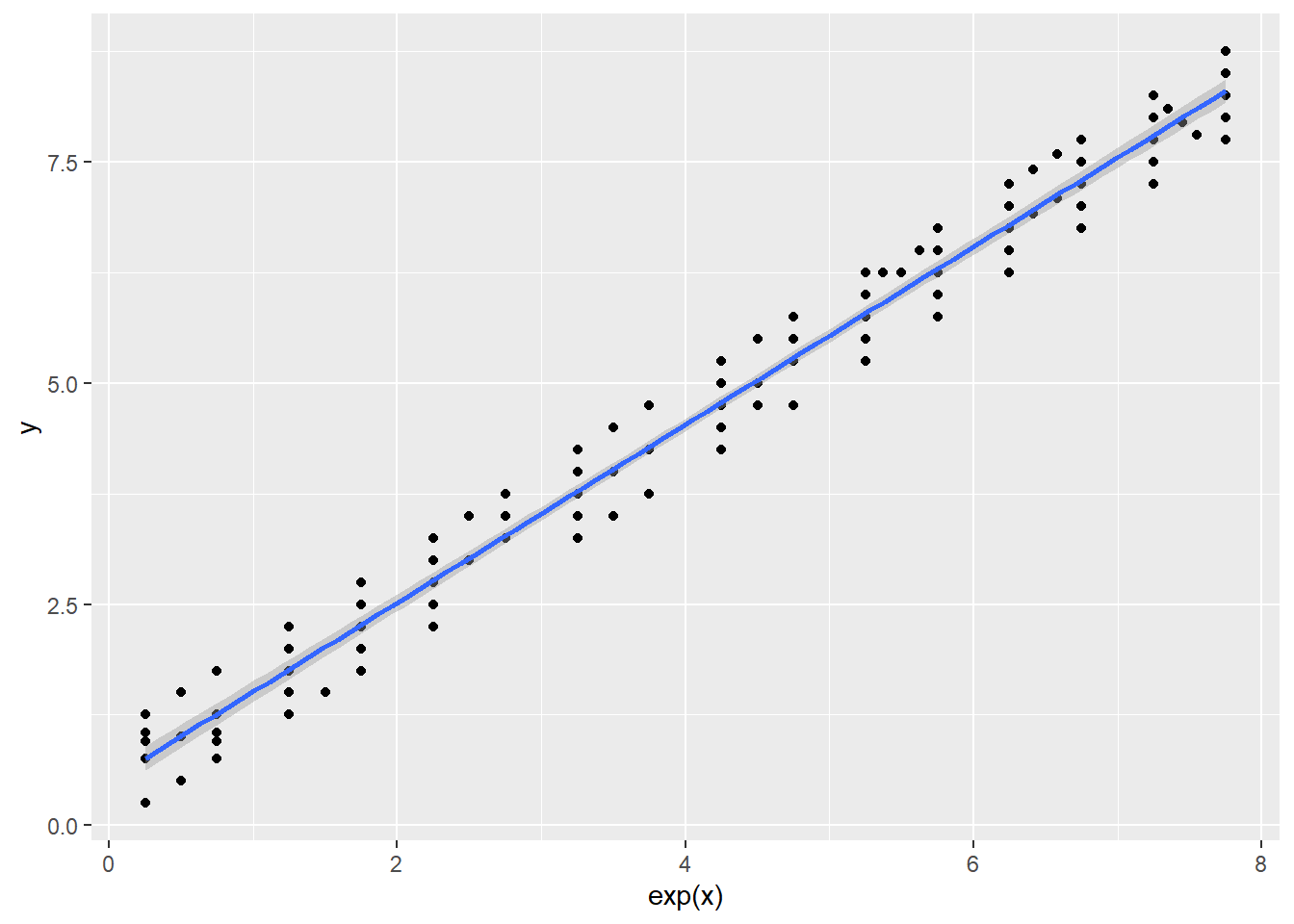
Data transformation come to rescue

data.lm2 <- lm(formula=y ~ exp(x), data = data1)
tab_model(data.lm2)

	y
Predictors	Estimates	CI	p
(Intercept)	0.51	0.36 – 0.65	<0.001
x [exp]	1.01	0.98 – 1.04	<0.001
Observations	100
R² / R² adjusted	0.977 / 0.977

ggplot(data=data1,  
       aes(x=exp(x), y=`y`)) +
  geom_point() +
  geom_smooth(method = lm)

`geom_smooth()` using formula = 'y ~ x'

The linearity assumption

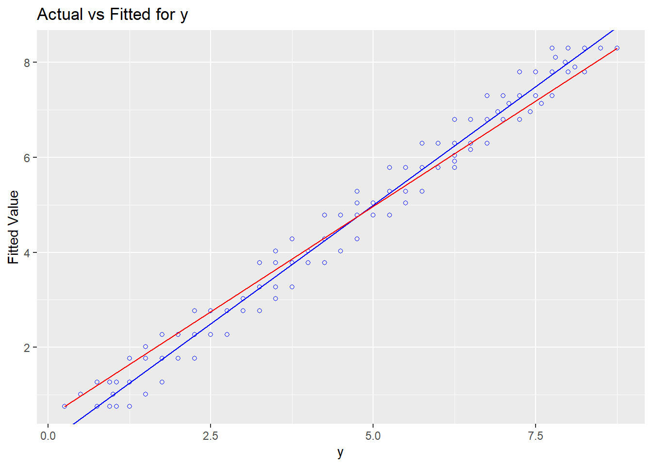
The diagnostic plot on the right shows that the linearity assumption has been conformed.

ols_plot_obs_fit(data.lm2, print_plot = TRUE)

The normality assumption

Warning

This is the test on the residual and not on the dependent variable.

Checking for serial correlation

The purpose of this test is to ensure the residuals of a multiple regression are time independent.

Spatial Non-stationary

When applied to spatial data, as can be seen, it assumes a stationary spatial process.
- The same stimulus provokes the same response in all parts of the study region.
- Highly untenable for spatial process.

Why do relationships vary spatially?

Sampling variation
- Nuisance variation, not real spatial non-stationarity.
Relationships intrinsically different across space
- Real spatial non-stationarity.
Model misspecification
- Can significant local variations be removed?

Some definitions

Spatial non-stationarity: the same stimulus provokes a different response in different parts of the study region.
Global models: statements about processes which are assumed to be stationary and as such are location independent.
Local models: spatial decompositions of global models, the results of local models are location dependent – a characteristic we usually anticipate from geographic (spatial) data.

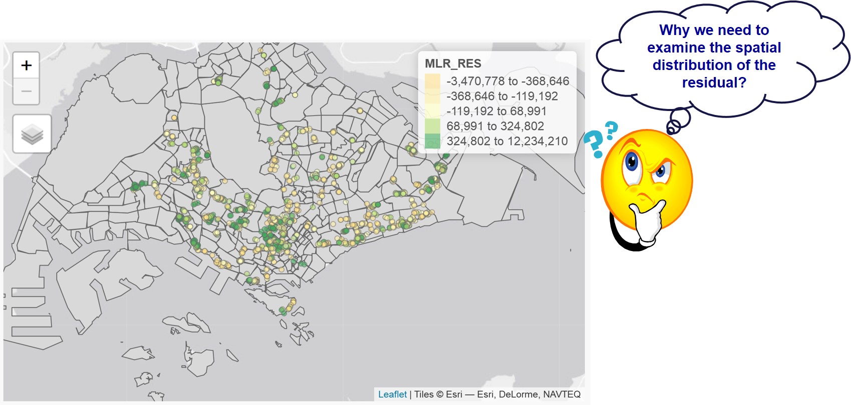
Spatial Autocorrelation assumption

The residuals are assumed to be distributed at random over geographical space.

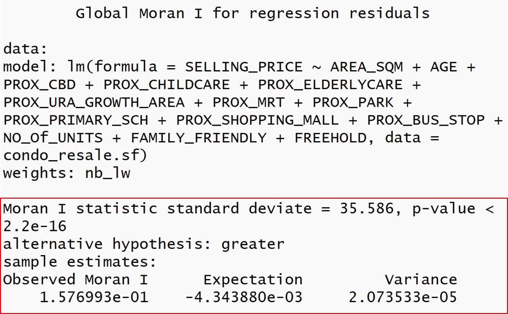
Test of spatial autocorrelation

To test if the relationships in the model are non-stationary.

lm.morantest() of spdep package will be used.

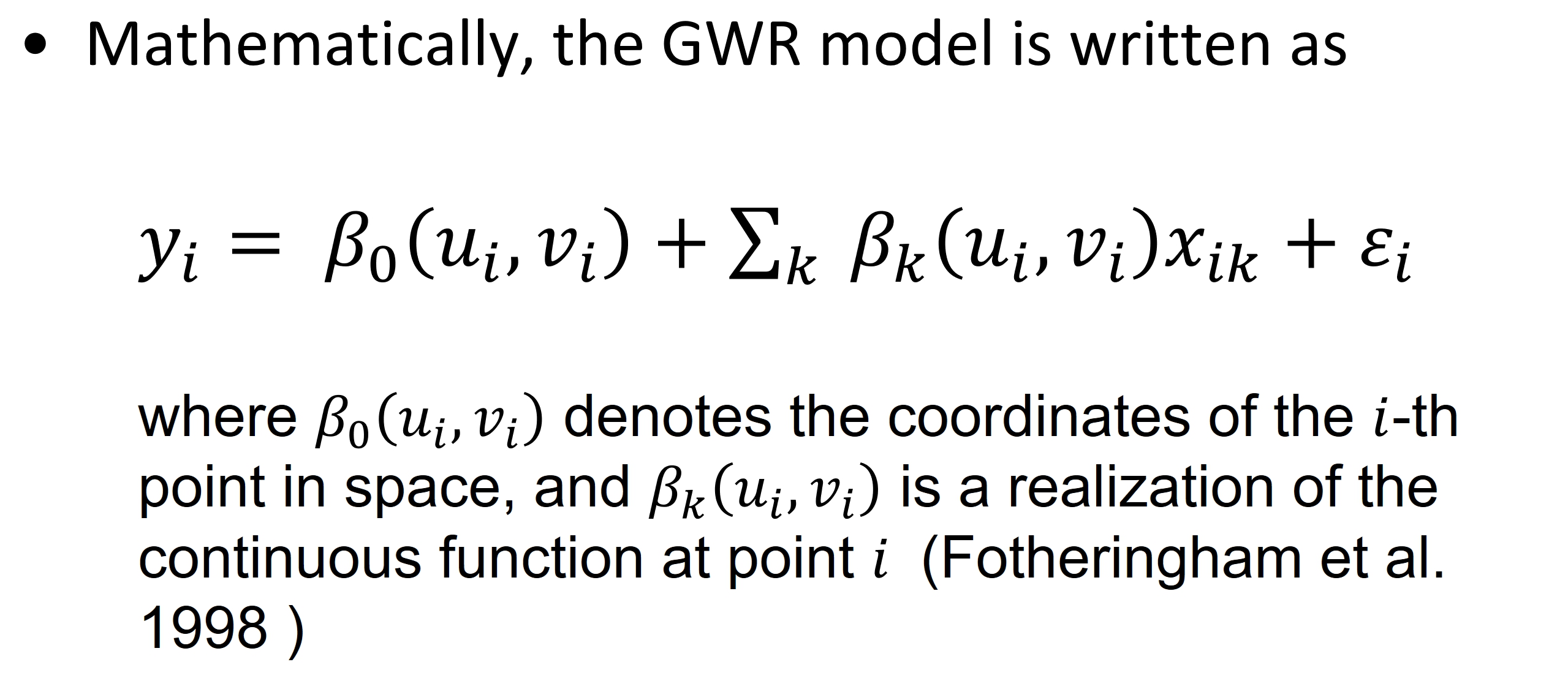
Geographically Weighted Regression (GWR)

Local statistical technique to analyze spatial variations in relationships.
Spatial non-stationarity is assumed and will be tested.
Based on the “First Law of Geography”: everything is related with everything else, but closer things are more related.

Geographically Weighted Regression (GWR): The method

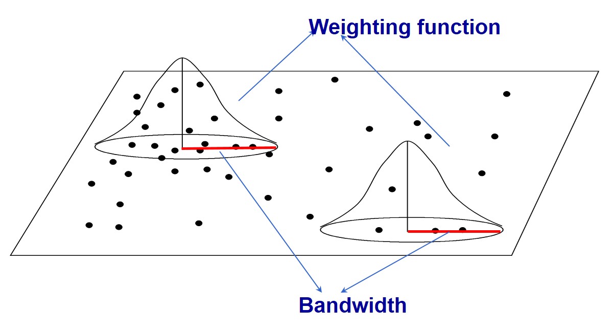
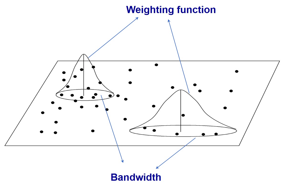
Calibration of GWR

Local weighted least squares
- Weights are attached with locations
- Based on the “First Law of Geography”: everything is related with everything else, but closer things are more related than remote ones

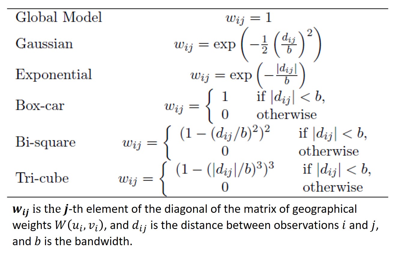
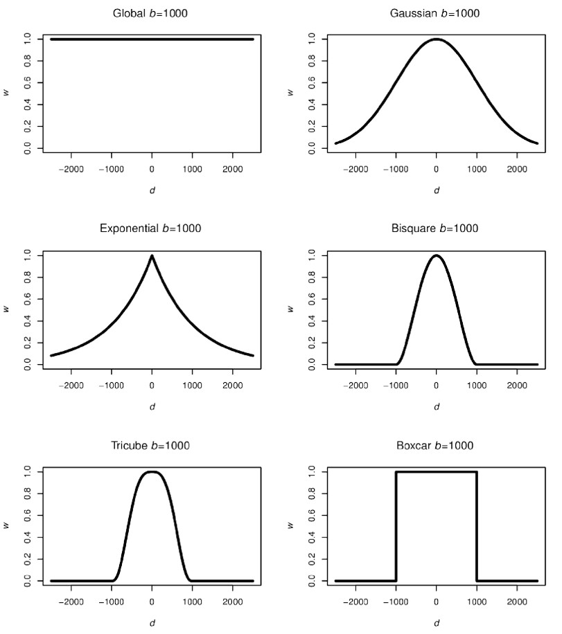
Calibration - Weighting functions

Calibration - Weighting schemes

Determines weights
- Most schemes tend to be Gaussian or Gaussian-like reflecting the type of dependency found in most spatial processes.
- It can be either Fixed or Adaptive.

Calibration - Determining Bandwidth

GWR Report

Package Model
Results of Global Regression
Results of Geographically Weighted Regression
SDF: A SpatialPointDataFrame

gwr: local R2

gwr: intercept

References

Brunsdon, C., Fotheringham, A.S., and Charlton, M. (2002) “Geographically weighted regression: A method for exploring spatial nonstationarity”. Geographical Analysis, 28: 281-289.

Brunsdon, C., Fotheringham, A.S. and Charlton, M., (1999) [“Some Notes on Parametric Significance Tests for Geographically Weighted Regression”](https://onlinelibrary-wiley-com.libproxy.smu.edu.sg/doi/abs/10.1111/0022-4146.00146. Journal of Regional Science, 39(3), 497-524.

Mennis, Jeremy (2006) “Mapping the Results of Geographically Weighted Regression”, The Cartographic Journal, Vol.43 (2), p.171-179.

Stephen A. Matthews ; Tse-Chuan Yang (2012) “Mapping the results of local statistics: Using geographically weighted regression”, Demographic Research, Vol.26, p.151-166.