Lesson 2: Wrangling Geospatial Data in R: sf approach and methods

Dr. Kam Tin Seong
Assoc. Professor of Information Systems(Practice)

School of Computing and Information Systems,
Singapore Management University

21 Feb 2023

Content

  • An overview of Geospatial Data Models

    • Vector and raster data model
    • Coordinate systems and map projection
  • Handling Geospatial Data in R: An Overview

  • Simple features approach

    • sf package

Geospatial Data Models

Why should we worry about?

Basic Spatial Data Models

  • Vector - implementation of discrete object conceptual model
    • Point, line and polygon representations.
    • Widely used in cartography, and network analysis.
  • Raster – implementation of field conceptual model
    • Array of cells used to represent objects.
    • Useful as background maps and for spatial analysis.

Vector Data Models

  • There are three basic geometric primitives, namely: points, lines (or polylines) and polygons.

Raster Data Models

  • All raster formats are basically the same
    • Cells organized in a matrix of rows and columns.
    • Content is more important than format: data or picture?

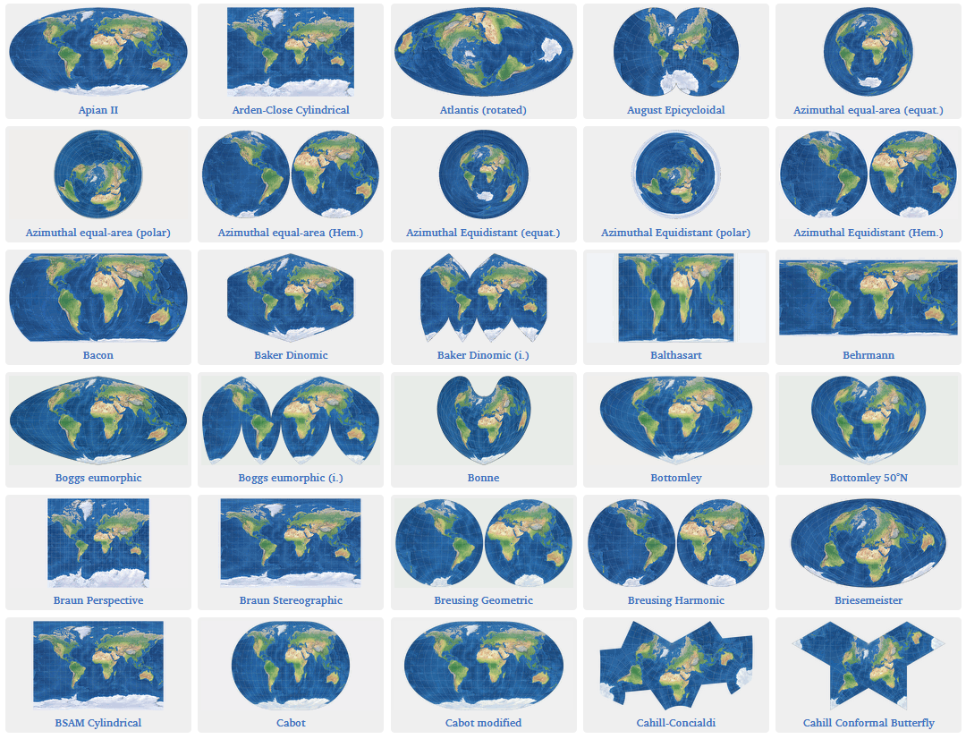
Coordinate Systems and Map Projections

What is a coordinate system?

A coordinate system is an important property of an geospatial data. It provides a location reference to the geospatial data.

  • There are two common types of coordinate systems used in mapping, namely: geographic coordinate systems and projected coordinate system.

Further Reading

Geographical Coordinate Systems

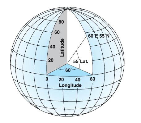
  • GCS define locations on the earth using a three-dimensional spherical surface. For example, WGS84.

  • They provides accuracy position information. Unit of measurement will be in either decimal degree or degree-minute-second format.

  • GCS, however, are not appropriate for distance and area measurements. In this figure, it is clear that 1 degree distance at the north pole is relatively shorter than 1 degree at the equator.
Further Reading

Projected Coordinate Systems (PCS)

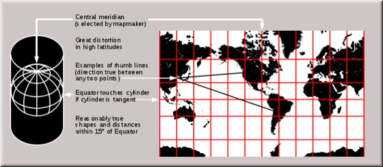
  • Based on a map projection such as transverse Mercator, Albers equal area, or Robinson.

  • PCS provides consistent length and area measurement across space. Hence, it is important to transform a geospatial data from GCS to PCS before performing geospatial analysis.
Further Reading

Singapore Projected Coordinate System

epsg.io provides a comprehensive list of country coordinate systems such as svy21.

Coordinates Reference Systems in R

  • In R, the notation used to describe the CRS is proj4string from the PROJ.4 library. It looks like this:

+proj=tmerc +lat_0=1.366666666666667 +lon_0=103.8333333333333 +k=1 +x_0=28001.642 +y_0=38744.572 +ellps=WGS84 +units=m +no_defs

  • This library is interfaced with R in the rgdal package, and the CRS class is defined partly in sp, partly in rgdal.
  • A CRS object is defined as a character NA string or a valid PROJ.4 CRS definition.

Standard for Geospatial Data Handling and Analysis

Further Reading

For more information, visit this link.

An introduction to simple features

  • feature: abstraction of real world phenomena (type or instance); has a geometry and other attributes (properties)

  • simple feature: feature with all geometric attributes described piecewise by straight line or planar interpolation between sets of points (no curves)

  • It is a hierarchical data model that simplifies geographic data by condensing a complex range of geographic forms into a single geometry class.

Simple features specification

  • Simple features specification is an open standard developed and endorsed by the Open Geospatial Consortium (OGC) to represent a wide range of geographic information.

Commonly used simple features

Simple Features: How they look like?

Simple Features: How they look like?

Simple Features: How they look like?

  • Geometry collection: GEOMETRYCOLLECTION (MULTIPOINT (5 2, 1 3, 3 4, 3 2), LINESTRING (1 5, 4 4, 4 1, 2 2, 3 2))

Geospatial Data Object Framework

  • To begin with, all contributed packages for handling spatial data in R had different representations of the data. This made it difficult to exchange data both within R between packages, and between R and external le formats and applications.

  • The first general package to provide classes and methods for spatial data types that was developed for R is called sp. It was first released on CRAN in 2005.

  • In late October 2016, sf was first released on CRAN to provide standardised support for vector data in R.

R packages that support spatial classes

In general, three R packages will be used to handle vector-based geospatial data in spatial classes, they are:

  • sp provides classes and methods for dealing with spatial data in R.

  • rgdal allows R to understand the structure of a geospatial data file by providing functions to read and convert geospatial data into easy-to-work-with R dataframes.

  • rgeos implements the methods of the OGC standard.

Introducing sf Package

  • sf package provides a syntax and data-structures which are coherent with the tidyverse.
  • A quick introduction can be found here.
  • For more detail, visit this link.

sf package dependencies

Source: Tidy spatial data analysis

sf & tidyverse

  • sf spatial objects are data.frames (or tibbles)
  • you can always un-sf, and work with tbl_df or data.frame having an sfc list-column
  • sf methods for filter, arrange, distinct, group_by, ungroup, mutate, select have sticky geometry
  • st_join() joins tables based on a spatial predicate
  • summarise unions geometry by group (or altogether)

What is so special about sf?

  • It builds upon the simple features standard (not R specific!), represents natively in R all 17 simple feature types for all dimensions (XY, XYZ, XYM, XYZM),
  • uses S3 classes: simple features are data.frame objects (or tibbles) that have a geometry list-column,
  • interfaces to GEOS to support the DE9-IM,
  • interfaces to GDAL with driver dependent dataset or layer creation options, Date and DateTime (POSIXct) columns, and coordinate reference system,
  • transformations through PROJ.4,
  • provides fast I/O with GDAL and GEOS using well-known-binary written in C++/Rcpp, and
  • directly reads from and writes to spatial databases such as PostGIS using DBI.

sfg : geometry for one feature

sf: objects with simple features

sf functions

  • Geospatial data handling

  • Geometric confirmation

  • Geometric operations

  • Geometry creation

  • Geometry operations

  • Geometric measurement

Geospatial data handling functions

  • st_read & read_sf: read simple features from file or database, or retrieve layer names and their geometry type(s)
  • st_write & write_sf: write simple features object to file or database
  • st_as_sf: convert a sf object from a non-geospatial tabular data frame
  • st_as_text: convert to Well Known Text(WKT)
  • st_as_binary: convert to Well Known Binary(WKB)
  • st_as_sfc: convert geometries to sfc (e.g., from WKT, WKB) as(x, “Spatial”): convert to Spatial*
  • st_transform(x, crs, …): convert coordinates of x to a different coordinate reference system
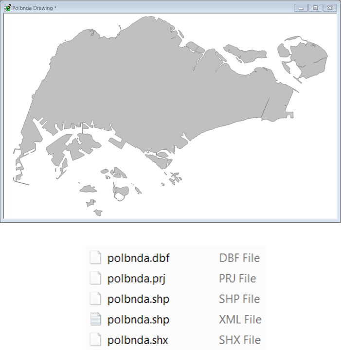
  • A shapefile is a simple, non-topological format for storing the geometric location and attribute information of geographic features.
  • Geographic features in a shapefile can be represented by points, lines, or polygons (areas).

Sample code chunk:

sf_mpsz = st_read(dsn = "data/geospatial", 
                  layer = "MP14_SUBZONE")

and

st_write(st_poly, "data/my_poly.shp")

Other vector GIS formats

  • MapInfo TAB format - MapInfo’s vector data format using TAB, DAT, ID and MAP files.
  • Personal Geodatabase - Esri’s closed, integrated vector data storage strategy using Microsoft’s Access MDB format
  • Keyhole Markup Language (KML) - XML based open standard (by OpenGIS) for GIS data exchange.
  • Geography Markup Language (GML) - XML based open standard (by OpenGIS) for GIS data exchange.
  • GeoJSON - a lightweight format based on JSON, used by many open source GIS packages.
  • TopoJSON, an extension of GeoJSON that encodes topology.

Sample code chunk to import kml file:

sf_preschool = st_read("data/geospatial/pre-schools-location-kml.kml")

Geometric confirmation

The commands below compare two sf data object and return a sparse matrix with matching (TRUE) indexes, or a full logical matrix.
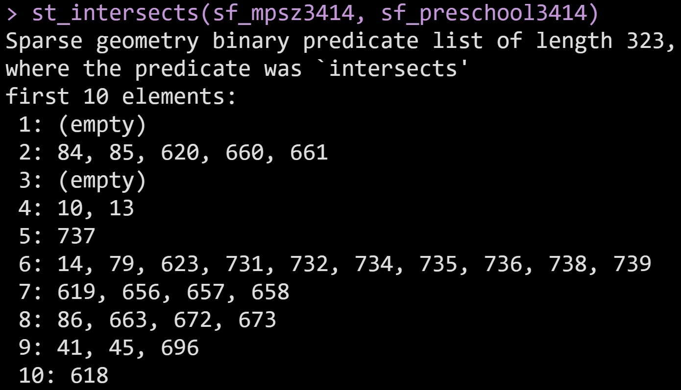
  • st_intersects: touch or overlap
  • st_disjoint: !intersects
  • st_touches: touch
  • st_crosses: cross (don’t touch)
  • st_within: within
  • st_contains: contains
  • st_overlaps: overlaps
  • st_covers: cover
  • st_covered_by: covered by
  • st_equals: equals
  • st_equals_exact: equals, with some fuzz returns a sparse (default) or dense logical matrix

Note

These functions return a logical matrix indicating whether each geometry pair meeting the logical operation.

sf Methods

Geometry generating logical operators

These commands overlay two sf data frames.
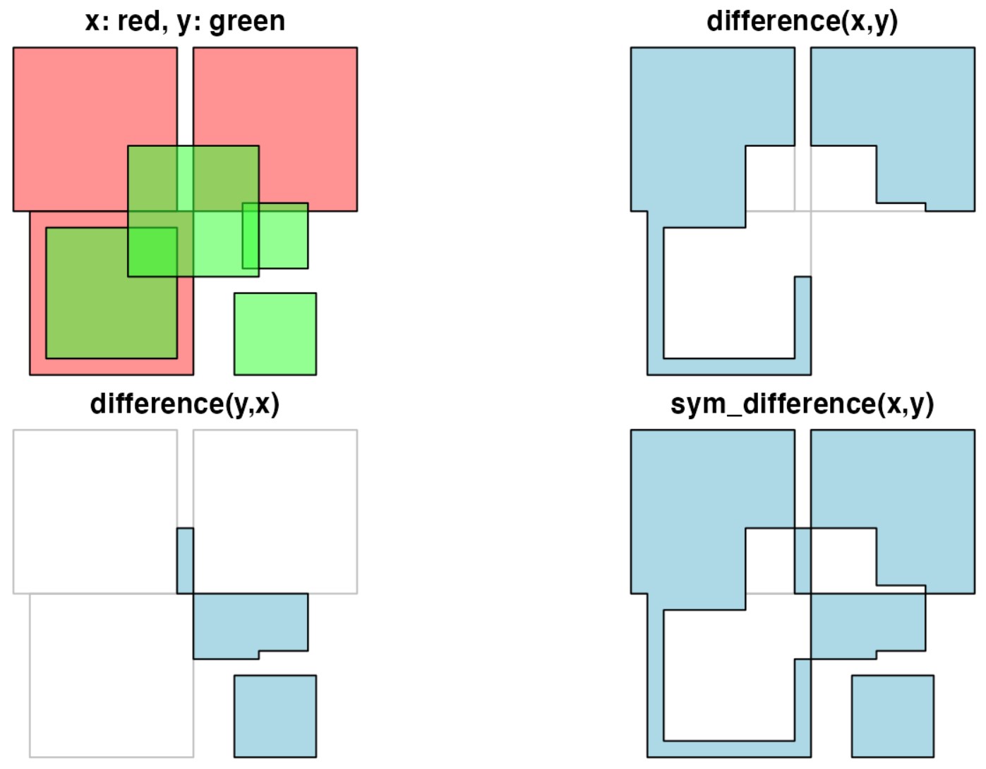
  • st_union: union of several geometries
  • st_intersection: intersection of pairs of geometries
  • st_difference: difference between pairs of geometries
  • st_sym_difference: symmetric difference (xor)

sf Methods

Higher-level operations: summarise, interpolate, aggregate, st_join

  • aggregate and summarise use st_union (by default) to group feature geometries
  • st_interpolate_aw: area-weighted interpolation, uses st_intersection to interpolate or redistribute attribute values, based on area of overlap:
  • st_join uses one of the logical binary geometry predicates (default: st_intersects) to join records in table pairs.
rd_joined = st_join(random_points, world) 

Manipulating geometries

The commands below perform unary operations on simple feature geometry sets.
  • st_line_merge: merges lines
  • st_segmentize: adds points to straight lines
  • st_voronoi: creates voronoi tesselation
  • st_centroid: gives centroid of geometry
  • st_convex_hull: creates convex hull of set of points
  • st_triangulate: triangulates set of points (not constrained)
  • st_polygonize: creates polygon from lines that form a closed ring
  • st_simplify: simplifies lines by removing vertices
  • st_split: split a polygon given line geometry
  • st_buffer: compute a buffer around this geometry/each geometry
  • st_make_valid: tries to make an invalid geometry valid (requires lwgeom)
  • st_boundary: return the boundary of a geometry
centroid_poly <- st_centroid(poly)

buf_poly <- st_buffer(poly, 5)

Convenience functions

  • st_zm: sets or removes z and/or m geometry
  • st_coordinates: retrieve coordinates in a matrix or data.frame
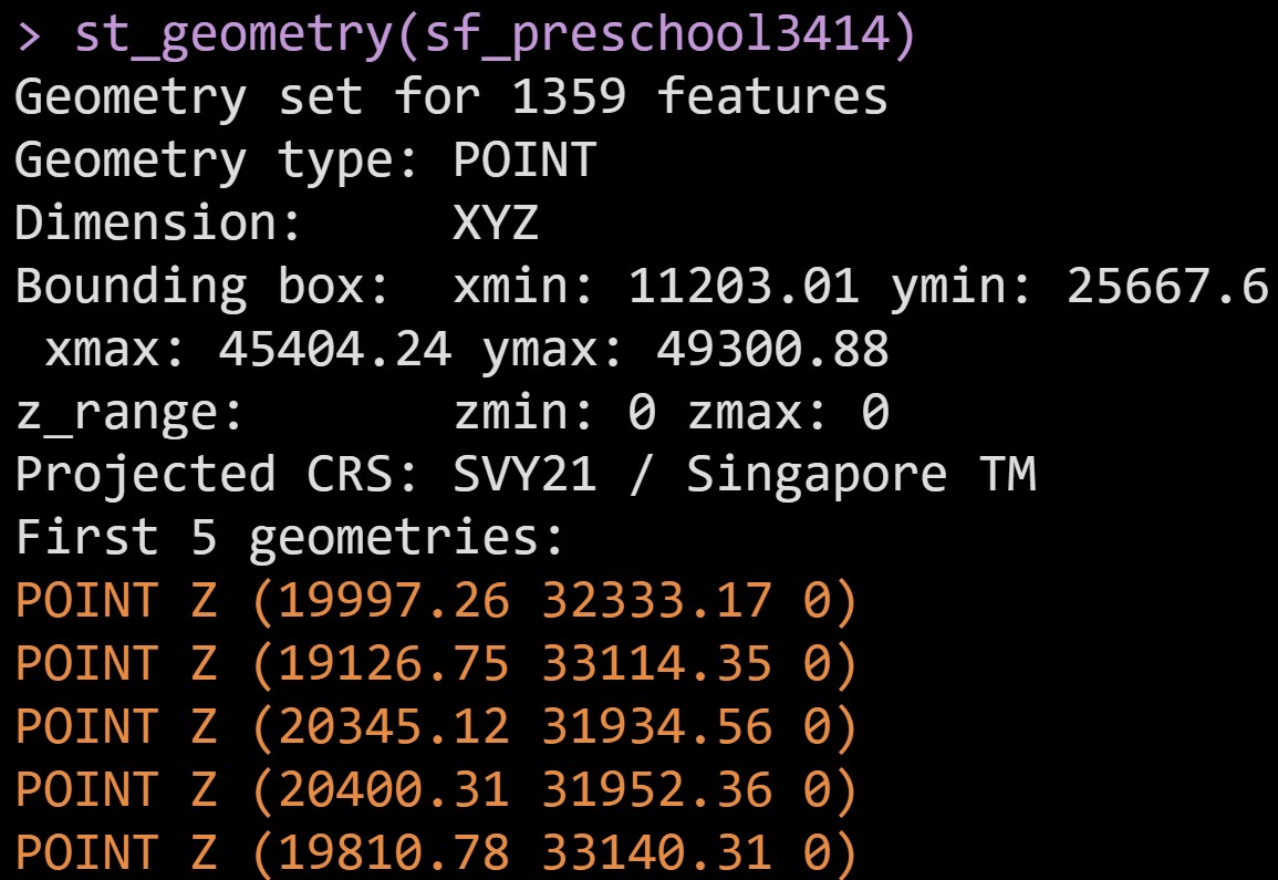
  • st_geometry: set, or retrieve sfc from an sf object
  • st_is: check whether geometry is of a particular type

References

All About sf package

Vignettes:

  1. Simple Features for R
  2. Reading, Writing and Converting Simple Features
  3. Manipulating Simple Feature Geometries
  4. Manipulating Simple Features
  5. Plotting Simple Features
  6. Miscellaneous
  7. Spherical geometry in sf using s2geometry

Others:

  1. R spatial follows GDAL and PROJ development